This article provides a comprehensive guide to initiate data analysis in R in 2025, tailored for beginners and written from the perspective of a non-native English speaker in Sri Lanka. We begin with setting up the R environment and proceed through essential data structures, data import/export, cleaning, exploratory data analysis (EDA), visualization, statistical modeling, machine learning with tidymodels, and reproducible reporting via R Markdown. We also introduce interactive dashboards with Shiny and recommend best practices for robust, maintainable workflows. Finally, a curated list of further learning resources is provided.
Introduction to R and Its Role in Data Analysis
R is a free, open-source programming language designed for statistical computing and graphics (RStudio, 2025)(posit.co). Since its inception in the mid-1990s, R has evolved into a powerhouse for data analysis, supported by a vibrant community and a rich ecosystem of packages (R For The Rest Of Us, 2025)(rfortherestofus.com). In 2025, R continues to lead in data science education and research owing to its versatility, extensive package repository, and emphasis on reproducibility (Posit, 2025)(posit.co).
Setting Up Your R Environment
Installing R and RStudio IDE
- Download R from the Comprehensive R Archive Network (CRAN). Choose the version appropriate for your operating system (CRAN, 2025).
- Install RStudio IDE, the most popular integrated development environment for R, offering code execution, syntax highlighting, and workspace management (Posit, 2025)(posit.co).
- Verify installation by opening RStudio and running:
versionYou should see output indicating R version 4.x or later (RStudio, 2025)(rfortherestofus.com).
RStudio Cloud and Server Options
For collaborative or cloud-based work, RStudio Cloud provides a browser-based interface, eliminating local installation hurdles (Posit, 2025)(posit.co). Enterprises may opt for Posit Workbench (formerly RStudio Server Pro) for multi-user deployments with advanced permissions (Mock, 2025)(posit.co).
Core Data Structures in R
R’s fundamental structures include:
- Vectors: One-dimensional, homogeneous data (e.g.,
numeric,character) (Wickham, 2025)(r4ds.had.co.nz). - Matrices: Two-dimensional, homogeneous (all elements same type).
- Data Frames: Two-dimensional, heterogenous; the standard for tabular data (DataCamp, 2025)(datacamp.com).
- Lists: Ordered collections of objects, enabling nested structures.
- Tibbles: Modern reimagining of data frames from the tibble package, with improved printing and subsetting (Tidyverse, 2025)(tidyverse.org).
Understanding these structures is vital for efficient data manipulation and analysis.
Data Import and Export
Reading Data
- CSV:
read.csv("file.csv")orreadr::read_csv("file.csv")for faster parsing (Tidyverse, 2025)(tidyverse.org). - Excel:
readxl::read_excel("file.xlsx")from the readxl package. - Databases: Use DBI and RSQLite or odbc for connecting to SQL databases.
Writing Data
- CSV:
write.csv(df, "output.csv"); readr counterpart:readr::write_csv(df, "output.csv")(Tidyverse, 2025)(tidyverse.org). - RDS:
saveRDS(df, "data.rds")for R-native serialization.
Effective import/export streamlines analysis workflows, enabling smooth transitions between R and other tools.
Data Cleaning and Preprocessing
Data cleaning is often the most time-consuming phase. Key steps include:
- Handling Missing Values: Identify with
is.na(), impute or remove records based on context (Wickham, 2025)(r4ds.had.co.nz). - Data Type Conversion: Ensure numeric, factor, or date formats as needed with
as.numeric(),as.factor(),lubridate::ymd(). - Outlier Detection: Use boxplots or z-scores; decide whether to transform, cap, or exclude (Wickham, 2025)(r4ds.had.co.nz).
- String Cleaning: Utilize stringr functions like
str_trim(),str_to_lower()for consistent text data (Tidyverse, 2025)(tidyverse.org). - Feature Engineering: Create new variables to capture domain insights, e.g.,
df$age_group <- cut(df$age, breaks=…).
The janitor package offers convenient functions like clean_names() and remove_empty() to accelerate these tasks.
Exploratory Data Analysis (EDA)
EDA uncovers patterns, anomalies, and hypotheses:
- Summary Statistics:
summary(df),dplyr::glimpse(df). - Univariate Analysis: Histograms (
ggplot2::geom_histogram()), density plots. - Bivariate Analysis: Scatterplots (
ggplot2::geom_point()), boxplots. - Correlation:
cor(df[numeric_cols]), visualized with corrplot.
Following Hadley Wickham’s guidance, iterative EDA fosters robust insights and informs subsequent modeling (Wickham, 2025)(r4ds.had.co.nz).
Data Visualization
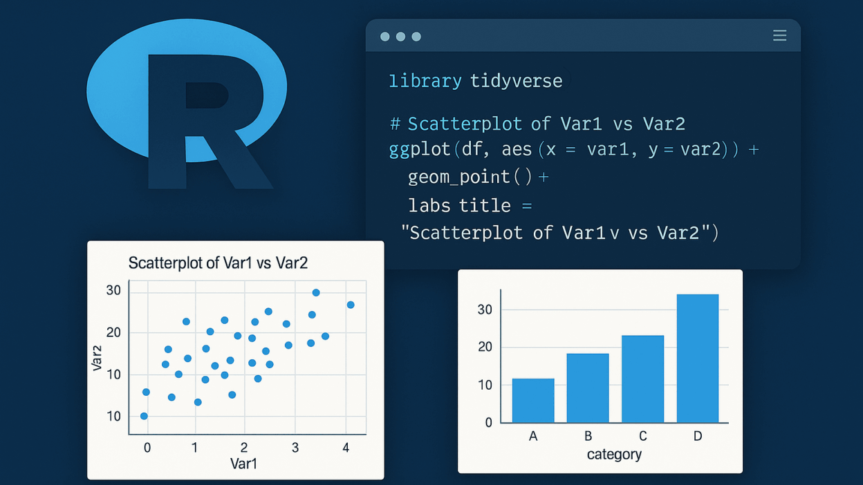
The ggplot2 package from the tidyverse offers a grammar of graphics:
library(ggplot2)
ggplot(df, aes(x = var1, y = var2, color = group)) +
  geom_point() +
  labs(title = "Scatterplot of Var1 vs Var2")
- Themes: Enhance appearance with
theme_minimal(),theme_classic(). - Faceting:
facet_wrap(~ category)for small multiples. - Interactive Plots: Use plotly to convert ggplots into interactive dashboards.
Visualization not only communicates results but also aids in deeper data understanding.
Statistical Analysis in R
R’s base and contributed packages support a wide range of statistical methods:
- Linear Models:
lm(y ~ x1 + x2, data = df); diagnostics viaplot(lm_object). - Generalized Linear Models:
glm(y ~ x, family = binomial, data = df)for logistic regression. - ANOVA:
aov(response ~ factor, data = df). - Time Series Analysis: forecast package:
auto.arima(),ets().
Statistical rigor, including assumption checks and effect sizes, is essential for credible findings.
Machine Learning with Tidymodels
The tidymodels framework unifies modeling workflows under tidy principles (Kuhn, 2025)(tidyverse.org):
library(tidymodels)
split <- initial_split(df, prop = 0.8)
train <- training(split); test <- testing(split)

rf_spec <- rand_forest() %>%
  set_engine("ranger") %>%
  set_mode("regression")

rf_workflow <- workflow() %>%
  add_recipe(recipe(target ~ ., data = train)) %>%
  add_model(rf_spec)

rf_fit <- rf_workflow %>%
  fit(data = train)
- Cross-Validation:
vfold_cv() - Tuning: tune package with grid/random search.
- Evaluation: Metrics via yardstick.
Tidymodels fosters reproducible, coherent pipelines from preprocessing to evaluation.
Reproducible Reporting with R Markdown
R Markdown combines narrative with executable R code (Posit Connect Docs, 2025)(docs.posit.co). A basic .Rmd document:
---
title: "Analysis Report"
output: html_document
---

```{r setup}
library(tidyverse)
summary(df)
- **Output Formats:** HTML, PDF, Word, slides.
- **Parameterization:** Build dynamic reports.
- **Publishing:** Deploy via **Posit Connect** or **GitHub Pages**.

This workflow ensures transparency and ease of collaboration.

## Interactive Dashboards with Shiny

**Shiny** enables web applications directly from R (ShinyConf, 2025):contentReference[oaicite:18]{index=18}:

```r
library(shiny)
ui <- fluidPage(
  titlePanel("My Shiny App"),
  sidebarLayout(
    sidebarPanel(sliderInput("n", "Sample size", 10, 100, 30)),
    mainPanel(plotOutput("hist"))
  )
)
server <- function(input, output) {
  output$hist <- renderPlot({
    hist(rnorm(input$n))
  })
}
shinyApp(ui, server)
Shiny apps facilitate real-time data exploration and stakeholder engagement without coding burden on end users.
Best Practices and Tips
- Version Control: Use Git and platforms like GitHub for collaboration and traceability (DataCamp, 2025)(datacamp.com).
- Project Organization: Leverage the {here} package and consistent directory structures.
- Code Style: Adopt the lintr package and follow tidyverse style guide (Tidyverse, 2025)(tidyverse.org).
- Documentation: Comment code and maintain a
README.md. - Automation: Use drake or targets for workflow management.
Adhering to these practices enhances productivity and reproducibility.
Further Learning Resources
- Official CRAN Task Views for comprehensive package listings (CRAN, 2025).
- R for Data Science by Hadley Wickham and Garrett Grolemund for foundational concepts (Wickham, 2025)(r4ds.had.co.nz).
- DataCamp’s R Track for structured online courses (DataCamp, 2025)(datacamp.com).
- Tidyverse Blog for updates on grammar of data manipulation and visualization (Tidyverse, 2025)(tidyverse.org).
- Shiny User Gallery for inspiration on interactive applications (ShinyConf, 2025)(shinyconf.com).
References
- CRAN (2025) The Comprehensive R Archive Network. Available at: https://cran.r-project.org/ (Accessed: June 2025).
- DataCamp (2025) How to Learn R From Scratch in 2025: An Expert Guide. Available at: https://www.datacamp.com/blog/learn-r (Accessed: June 2025).
- Kuhn, M. (2025) ‘Q1 2025 tidymodels digest’, Tidyverse Blog, 27 February. Available at: https://www.tidyverse.org/blog/2025/02/tidymodels-2025-q1/ (Accessed: June 2025).
- Mock, T. (2025) ‘RStudio IDE and Posit Workbench 2025.05.0: What’s New’, Posit Blog. Available at: https://posit.co/blog/rstudio-2025-05-0-whats-new/ (Accessed: June 2025).
- Posit (2025) Download RStudio. Available at: https://posit.co/downloads/ (Accessed: June 2025).
- Posit Connect Docs (2025) R Markdown – Posit Connect Documentation Version 2025.05.0. Available at: https://docs.posit.co/connect/user/rmarkdown/ (Accessed: June 2025).
- R For The Rest Of Us (2025) What’s New in R: March 3, 2025, Available at: https://rfortherestofus.com/2025/03/whats-new-in-r-march-3-2025 (Accessed: June 2025).
- RStudio (2025) R Weekly 2025-W19, Top 40 New CRAN Packages, recipes, 30 Day Chart Challenge, Rotation with Modulo, Available at: https://rweekly.org/2025-W19.html (Accessed: June 2025).
- ShinyConf (2025) ShinyConf 2025: Shine On with Shiny!. Available at: https://www.shinyconf.com/ (Accessed: June 2025).
- Tidyverse (2025) Posts – Tidyverse. Available at: https://www.tidyverse.org/blog/ (Accessed: June 2025).
- Wickham, H. (2025) 7 Exploratory Data Analysis – R for Data Science. Available at: https://r4ds.had.co.nz/exploratory-data-analysis.html (Accessed: June 2025).


